
pgvector is excellent. It is also, at large scale, expensive — because the HNSW index it gives you wants to live in memory to be fast, and “wants to live in memory” stops being a casual statement somewhere around fifty million 1536-dimensional embeddings. At which point you reach for Pinecone, or you scale up the box, or you wave your hands about sharding, or you find out about pgvectorscale.
This post is about the fourth option.
A note on names
pgvectorscale comes from Tiger Data, which is the company formerly known as Timescale. The rebrand happened in June 2025 along with a shift in framing: they are no longer pitching themselves primarily as a time-series database company but as the “fastest PostgreSQL,” with TimescaleDB demoted from headline product to one extension among several. The other extensions in the family are pgvectorscale (the subject of this post), pgai (LLM utilities), and pg_textsearch (a recent BM25 implementation that becomes important later).
The PostgreSQL community was mildly amused by the naming — TigerBeetle, TigerGraph, and WiredTiger were all already taken — but none of that matters for the technology, which is good.
What pgvector gives you
The baseline. pgvector is a PostgreSQL extension that adds a vector type and three index strategies: exact (no index), ivfflat (cluster-based ANN), and hnsw (graph-based ANN, added in 0.5.0). HNSW won the production fight on quality grounds and is what most people use at scale. Its problem, which is structural rather than fixable, is that the graph wants to be resident in shared_buffers (or at least the OS page cache) for queries to be fast. Pages full of vectors are large, queries traverse them in a pattern that is nearly the worst case for an LRU buffer, and once the working set exceeds RAM, p95 latency falls off a cliff.
Current pgvector is 0.8.2 (February 2026), which is a security release fixing CVE-2026-3172 — a buffer overflow in parallel HNSW index builds that can leak data from other relations or crash the backend. If you’re on anything from 0.6.0 (when parallel HNSW landed) through 0.8.1 and you’ve ever run CREATE INDEX ... USING hnsw without first setting max_parallel_maintenance_workers = 0, upgrade. The substantive feature work was in 0.8.0, which added iterative index scans (hnsw.iterative_scan, ivfflat.iterative_scan) to mitigate the “I asked for ten results and got three” failure mode that happens when you stack a WHERE clause on top of an ANN query. Useful, but a workaround for the same underlying memory-residency problem: ANN indexes hate being post-filtered.
What pgvectorscale adds
Three things, in decreasing order of how much you’ll care:
StreamingDiskANN. A new index type — written USING diskann in CREATE INDEX — based on Microsoft Research’s DiskANN. The point of DiskANN is right there in the name: it is an ANN graph designed to live on SSD rather than in memory. The graph traversal is structured so the I/O pattern is friendly to disk, the in-memory footprint is small (just compressed vectors used for distance approximation during traversal), and full-fidelity vectors are read from disk only for the reranking step at the end of the search. The “Streaming” prefix is Tiger Data’s contribution: the index supports streaming results out under relaxed ordering, which is the same trick pgvector’s iterative scans use, just done correctly from the start instead of bolted on.
Statistical Binary Quantization (SBQ). A compression scheme. Standard binary quantization throws away everything except the sign bit per dimension, which works surprisingly well but loses information. SBQ uses 1–2 bits per dimension (defaulting to 2 below 900 dimensions, 1 above) with a statistical encoding that improves recall over plain BQ. The compressed vectors live in memory and are used for fast distance approximation during graph traversal; the full vectors stay on disk and are read only for reranking. This is what makes the in-memory footprint small enough to keep cache hit rates high without storing everything.
Label-based filtering. Based on Microsoft’s Filtered DiskANN paper. You attach a smallint[] array of labels to each row, include it in the index, and filter using the array overlap operator &&. The index handles filtering during traversal rather than as a post-filter, which matters because post-filtering an ANN index is the leading cause of “why am I getting only three results when I asked for ten” in production vector search. Labels have to fit in smallint (-32768 to 32767), which is enough for most categorical filtering use cases and not enough for anything that’s really a foreign key.
The current release is 0.9.0 (November 2025), which added parallel index builds — important if you’ve ever waited four hours for an HNSW build on fifty million rows and started questioning your life choices. Parallel builds require SBQ storage, no labels, and at least 65,536 vectors by default. PostgreSQL 18 is supported.
A small benchmark
I wanted my own numbers, on hardware I could afford to leave running. The setup:
- Linode
g6-standard-2: 2 vCPU, 3.8 GB RAM - PostgreSQL 16.13,
shared_buffers=1GB,effective_cache_size=2GB pgvector0.8.0,pgvectorscale0.5.1 (the 0.8.2 fixes are CVE and packaging only — they don’t move the latency numbers)- 1 million 1536-dimensional vectors, cosine distance
- Recall@10, single-stream and concurrent-2
This is the memory-constrained regime — the HNSW index ends up at 8.19 GB and does not fit in shared_buffers, effective_cache_size, or any other cache that matters. That is exactly the regime where DiskANN’s design is supposed to pay off.
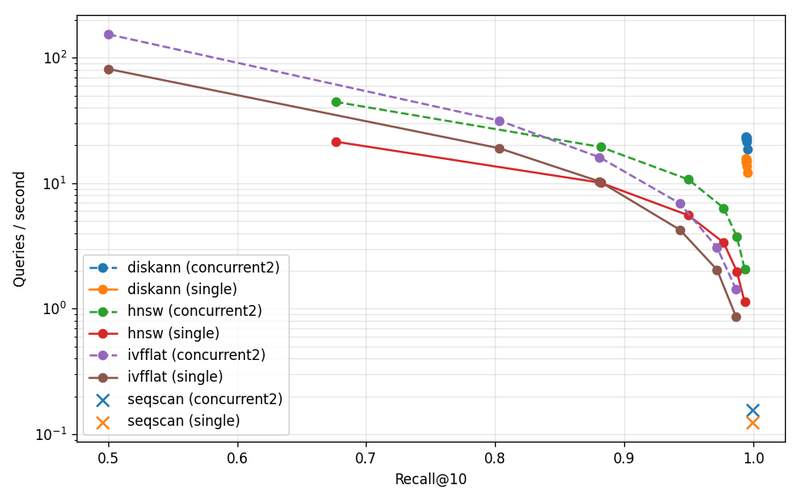
A note on operating points: each ANN index gets a parameter sweep, and I report the row whose recall lands closest to 0.99. DiskANN’s whole sweep stayed at ~0.9945 — the parameter knob barely moves recall at this scale — so I report the lowest-recall row from its sweep. HNSW’s sweep topped out at 0.9934 and never quite reached 0.99; the table interpolates between bracketing points. IVFFlat never reached 0.99 in the sweep at all, so it’s excluded from the headline.
| Index | p95 latency (ms, single) | QPS (concurrent-2) | Recall@10 |
|---|---|---|---|
diskann |
178.7 | 22.9 | 0.9945 |
hnsw |
1603.8 | 3.0 | 0.9900 |
seqscan |
8847.4 | 0.2 | 0.9997 |
DiskANN is 9.0× faster than HNSW at p95 single-stream, and 7.6× higher throughput under concurrent-2, at matched recall. Sequential scan still wins on recall — it always will — and gets murdered on latency, also as expected.
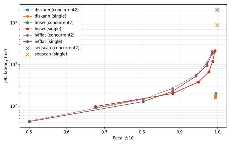
The recall-vs-p95 plot is the one to look at. The DiskANN points cluster in a tight knot in the lower-right corner — high recall, low latency, parameter sweep does almost nothing. HNSW and IVFFlat trace classic recall-latency tradeoff curves: to push HNSW past 99% recall you pay an order of magnitude in latency. The flat DiskANN behavior is what you want from a production index. Tune for recall, get latency for free.
The concurrent-2 results are also informative: HNSW concurrent-2 is slower than HNSW single-stream at the high-recall operating point, because two query streams compete for the same too-small page cache and thrash. DiskANN concurrent-2 holds up because the working set actually fits.
The build cost story is just as lopsided:
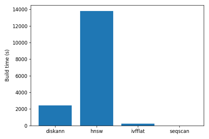
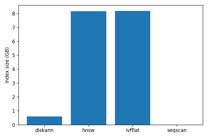
| Index | Build time | Index size |
|---|---|---|
diskann |
40 minutes | 0.59 GB |
hnsw |
3.8 hours | 8.19 GB |
ivfflat |
4 minutes | 8.20 GB |
DiskANN’s index is 14× smaller than HNSW’s. That is the entire point of SBQ: the part that has to live in memory is small, and the full vectors stay on disk to be read only at reranking time. HNSW has no such trick — graph nodes contain full vectors and the whole structure has to be paged in to be fast. IVFFlat is fast to build because it does much less work, and pays for it in recall.
Caveats: this is 1M vectors, not 50M; one hardware class, not a sweep; cosine only; read-only after load; no Pinecone or Qdrant or Weaviate in the comparison. For larger-scale numbers and head-to-head against managed vector databases, Tiger Data’s own benchmark on 50M 768-dimensional Cohere embeddings against Pinecone’s storage-optimized tier is the reference — vendor-skepticism applies, methodology is documented, and the directional finding matches what I see at smaller scale. The point of running my own benchmark wasn’t to reproduce the headline. It was to confirm that the design works on cheap hardware in the regime where it should win. It does, by a wide margin.
Why this is implemented in Rust
A digression, but a useful one — and one I’m including because the readership of this blog skews toward people who have heard of Rust but haven’t necessarily written a PostgreSQL extension in it.
pgvector is C, the way every PostgreSQL extension has historically been C. pgvectorscale is Rust, built on the pgrx framework. pgrx handles the FFI dance between Rust and PostgreSQL’s C structures: the MemoryContext system that PostgreSQL uses instead of malloc/free, the SPI interface for executing SQL from inside an extension, the PG_FUNCTION_ARGS macro and its arity-checking, the access-method API (IndexAmRoutine) that you have to implement to define a new index type. Rust’s borrow checker doesn’t help you across the FFI boundary, so pgrx wraps the unsafe parts in safe abstractions and uses macros to generate the C-compatible exports.
The user-facing consequence is nothing: CREATE EXTENSION vectorscale CASCADE; and you have a diskann access method. The maintainer-facing consequence is that the implementation is in a memory-safe language with sum types, traits, and a usable error system, which means a different and (I think) larger pool of people can plausibly contribute to it. If you’ve been waiting for a reason to read Rust, browsing the pgvectorscale source is a good one — the index access-method implementation is in src/access_method/, and the SBQ encoding is in src/access_method/sbq.rs, and both are reasonably approachable.
The other consequence is that building the extension requires cargo and cargo-pgrx, not just make. If you maintain a deployment pipeline that bakes extension binaries into images, this is a one-time annoyance.
Hybrid search, briefly
Vector search finds things that mean similar things. Lexical search finds things that contain the same words. They fail in opposite directions: vector search confidently returns “Toyota Camry” when you asked for the SKU PROD-SKU-7842X; lexical search confidently returns nothing when you asked for “automobile” and the corpus says “car.”
The standard fix is to run both searches and fuse the results. The standard fusion algorithm is Reciprocal Rank Fusion, which is embarrassingly simple: each retriever produces a ranked list, each document gets a score of 1 / (k + rank) from each retriever it appears in, scores are summed, the list is re-sorted. k defaults to 60. RRF works because it only cares about ranks, not raw scores — which means it doesn’t need normalization across retrievers that produce wildly different score distributions (cosine distances live in [0, 2], BM25 scores live in “however large your query and document happen to be”).
For the lexical side, you have two reasonable choices: PostgreSQL’s built-in tsvector with ts_rank (works everywhere, weaker ranking than BM25), or Tiger Data’s pg_textsearch extension (proper BM25, requires you to install it; v1.0.0 shipped in March 2026). I’m going to use tsvector here because it works in any vanilla PostgreSQL — drop in pg_textsearch if you have it.
A concrete example
Suppose you have a corpus of documents with embeddings already generated. The schema:
1 CREATE EXTENSION IF NOT EXISTS vectorscale CASCADE; 2 3 CREATE TABLE documents ( 4 id BIGINT PRIMARY KEY GENERATED BY DEFAULT AS IDENTITY, 5 title TEXT NOT NULL, 6 content TEXT NOT NULL, 7 embedding VECTOR(1536) NOT NULL, 8 content_tsv TSVECTOR GENERATED ALWAYS AS ( 9 setweight(to_tsvector('english', title), 'A') || 10 setweight(to_tsvector('english', content), 'B') 11 ) STORED 12 ); 13 14 CREATE INDEX documents_embedding_idx 15 ON documents USING diskann (embedding vector_cosine_ops); 16 17 CREATE INDEX documents_tsv_idx 18 ON documents USING GIN (content_tsv);
The tsvector is generated and stored; you don’t maintain it manually. Title gets weight A, body gets weight B, so a hit in the title outranks a hit in the body — which is what you want. The DiskANN index uses cosine distance, which is what every embedding model worth using is calibrated for.
Now the Python. I am using psycopg (version 3, not psycopg2), and the canonical pgvector Python client. Embedding generation is left to your imagination; assume embed(text) -> list[float] returns a 1536-dimensional vector from whatever model you’re using:
1 import psycopg 2 from pgvector.psycopg import register_vector 3 4 # RRF parameters. k=60 is the value from the original paper; it is 5 # almost never worth tuning unless you have a strong empirical reason. 6 RRF_K = 60 7 CANDIDATE_LIMIT = 100 # How many candidates each retriever returns. 8 FINAL_LIMIT = 10 # How many results we return to the caller. 9 10 11 def hybrid_search( 12 conn: psycopg.Connection, 13 query: str, 14 limit: int = FINAL_LIMIT, 15 ) -> list[tuple[int, float]]: 16 """Run lexical and vector search, fuse with RRF, return top `limit` IDs.""" 17 18 query_vec = embed(query) 19 20 with conn.cursor() as cur: 21 # Transaction-local rescore knob. Higher values trade latency 22 # for recall; 50 is the default, 200-400 is reasonable for 23 # quality-sensitive workloads. 24 cur.execute("BEGIN") 25 cur.execute("SET LOCAL diskann.query_rescore = 50") 26 27 # Lexical: ts_rank against websearch_to_tsquery, which handles 28 # quoted phrases, AND/OR, and exclusion (-word) without you 29 # having to parse anything yourself. 30 cur.execute( 31 """ 32 SELECT id 33 FROM documents, websearch_to_tsquery('english', %s) AS q 34 WHERE content_tsv @@ q 35 ORDER BY ts_rank(content_tsv, q) DESC 36 LIMIT %s 37 """, 38 (query, CANDIDATE_LIMIT), 39 ) 40 lexical_ids = [row[0] for row in cur.fetchall()] 41 42 # Semantic: cosine distance against the DiskANN index. 43 cur.execute( 44 """ 45 SELECT id 46 FROM documents 47 ORDER BY embedding <=> %s::vector 48 LIMIT %s 49 """, 50 (query_vec, CANDIDATE_LIMIT), 51 ) 52 semantic_ids = [row[0] for row in cur.fetchall()] 53 54 cur.execute("COMMIT") 55 56 return reciprocal_rank_fusion(lexical_ids, semantic_ids, limit) 57 58 59 def reciprocal_rank_fusion( 60 lexical_ids: list[int], 61 semantic_ids: list[int], 62 limit: int, 63 ) -> list[tuple[int, float]]: 64 """Combine two ranked lists by RRF. Inputs are document IDs in 65 retriever-defined sort order — best result first. Only rank 66 position matters; raw scores are discarded by design.""" 67 scores: dict[int, float] = {} 68 69 for rank, doc_id in enumerate(lexical_ids): 70 scores[doc_id] = scores.get(doc_id, 0.0) + 1.0 / (RRF_K + rank + 1) 71 72 for rank, doc_id in enumerate(semantic_ids): 73 scores[doc_id] = scores.get(doc_id, 0.0) + 1.0 / (RRF_K + rank + 1) 74 75 return sorted(scores.items(), key=lambda kv: kv[1], reverse=True)[:limit] 76 77 78 def main(): 79 with psycopg.connect("dbname=mydb") as conn: 80 register_vector(conn) 81 results = hybrid_search(conn, "how do I tune autovacuum on a large table") 82 for doc_id, score in results: 83 print(f"{doc_id}: {score:.4f}")
A few notes on the choices in that code:
websearch_to_tsquery, notplainto_tsquery. The former handles quoted phrases ("exact match"), exclusion (-word), andAND/ORnaturally. The latter doesn’t. There is no reason to useplainto_tsqueryin modern code.SET LOCAL diskann.query_rescoreinside a transaction, not session-levelSET. The transaction-local form means you don’t pollute connection-pooled sessions with leftover GUC settings that bleed into other queries. Always preferSET LOCALinside connection-pooled applications.- RRF runs client-side. You can do it in SQL — there are blog posts that do — but the pure-SQL versions are unreadable, fragile under schema changes, and don’t compose well when you want to add a third retriever (a cross-encoder reranker, say). Twenty lines of Python stays understandable.
- Two sequential queries on one connection, not parallel. For most workloads, the latency win from running them on separate connections isn’t worth the connection-pool complexity. If you’re running this at high QPS and have measured that the sequential round-trip is the bottleneck, switch to
asyncioand run them concurrently. Don’t do it preemptively. - No reranker. A common production pipeline adds a cross-encoder reranker (
bge-reranker, Cohere Rerank) on top of the RRF output. For small N, this is cheap and meaningfully improves quality. I’ve left it out to keep the example focused. If you go to production, you should probably add one.
When to actually use this
If your vector index fits comfortably in shared_buffers plus filesystem cache and your throughput is fine, stay on pgvector HNSW. It is structurally faster than DiskANN when the whole graph is RAM-resident — DiskANN always pays at least one disk read at the rerank step — and the operational simplicity of fewer extensions matters.
pgvectorscale becomes interesting when one of these is true:
- The index doesn’t fit in RAM and you don’t want to pay for an instance large enough to make it fit. The benchmark above is the concrete version of this argument: a 4 GB Linode, an 8 GB HNSW index, and a 9× latency penalty at the operating point. Scale up the corpus or scale down the box and the gap widens.
- You have selective metadata filters that destroy HNSW recall, and you can express the filter as a
smallint[]of labels. - You’re considering a dedicated vector database to escape the first two, and you’d rather not run two databases.
The third case is where the Tiger Data marketing is aimed, and where their Pinecone benchmarks are most relevant. The argument — that you should not run two databases when one will do — is correct on the merits, even when delivered with the volume turned up.